Computer vision models for infrastructure defect detection are only as good as the data they were trained on. This post describes the decisions that go into building a training dataset for power infrastructure inspection: annotation taxonomy, handling rare defect classes, managing the difference between early-stage and late-stage deterioration, and the tradeoffs we made in dataset construction.
Why Infrastructure Defect Data Is Different From General Vision Data
Generic image recognition datasets are large, diverse, and cover categories that appear in roughly equal frequency. Defect detection for transmission steel and pipeline surfaces is different along almost every dimension that matters for machine learning.
The classes are heavily imbalanced. A well-maintained structure has very few actively deteriorating members. Early-stage pitting, which is the most important class to catch because it is actionable before structural risk develops, is sparse relative to intact surface area. Coating delamination is more common than active corrosion in early inspection of younger infrastructure. Fatigue crack propagation at weld seams is rare even on aging structures. Building a balanced training set requires deliberate oversampling strategies for the rare classes and augmentation approaches that preserve the morphological characteristics that distinguish early-stage from late-stage presentation.
There is also a domain shift problem. Transmission steel is galvanized, and the appearance of corroded galvanized steel is different from the appearance of painted or bare steel corrosion that dominates publicly available industrial inspection datasets. The zinc layer on galvanized steel oxidizes to zinc carbonate before the underlying steel substrate begins corroding, which creates a white powdery surface change that precedes the familiar orange-red iron oxide appearance. A model trained on datasets that predominantly contain rusted bare steel will not learn to recognize early-stage galvanic corrosion on transmission infrastructure until the corrosion has already reached an advanced stage.
Defining the Annotation Taxonomy Before Collecting Images
The annotation taxonomy has to be defined before data collection begins, not after. This sounds obvious but is regularly reversed in practice. The typical pattern is to collect a large volume of images, then figure out what labels to apply. That approach produces datasets with internally inconsistent labeling because annotators working without a clear taxonomy will make different decisions on ambiguous cases at different times.
Our taxonomy for transmission steel surfaces uses five base classes. Surface pitting covers localized depressions in the metal substrate from galvanic or atmospheric corrosion initiation. Oxidation banding covers the characteristic band patterns that develop at galvanic transition zones, particularly where dissimilar metals are in contact such as at bolt seats and hardware attachment points. Fatigue crack propagation covers the linear and branching fracture patterns that initiate at weld seams or geometric stress concentrators under repeated load cycling. Coating failure covers delamination, blistering, and adhesion loss before the underlying metal is exposed. Mechanical joint wear covers bolt-seat corrosion, thread damage, and fitting degradation indicators at structural connection hardware.
These five classes are not exhaustive of everything that can go wrong with transmission infrastructure. They are the set of defect morphologies that are detectable from imagery at the standoff distances and illumination conditions a robot inspection platform can provide, and that are actionable by maintenance teams when flagged. Classes that are not detectable under inspection conditions or that would not change a maintenance decision are not useful annotation targets regardless of how interesting they are from a materials-science perspective.
Handling Rare Classes Without Fabricating Examples
Fatigue crack propagation in particular is rare in the image data we have collected. Most transmission infrastructure, even on older towers, does not show active crack propagation in any given inspection period. This creates a practical problem: the model needs enough examples of crack patterns to learn their distinctive morphological signatures, but we do not have enough naturally occurring examples to train on without augmentation.
The augmentation approaches that work for rare classes in this domain are constrained. Geometric augmentation (rotation, flip, crop) does not add useful variation because the morphological signatures are not orientation-dependent at the scale of variation geometric transforms provide. Color jitter and noise augmentation can help with generalization across different imaging conditions but does not expand the sample of morphological variation itself.
What we found more useful is augmenting at the structural level: sourcing additional images of crack morphology from related contexts, specifically weld inspection imagery from the industrial NDT literature, that share the relevant morphological features even if the surrounding material and context differ. This requires careful curation to ensure the augmented examples do not introduce false patterns that are only present in the source domain. The annotation for augmented examples needs to be reviewed by someone who understands both the augmentation source and the target domain.
Generating synthetic examples using procedural rendering is an option we have explored but not yet used in the main training pipeline. The quality of synthetic surface defect imagery has improved significantly with recent advances in material rendering, but validating that synthetic examples faithfully represent real defect morphology requires a matching set of real examples to compare against. The validation problem is hardest to solve for exactly the rare classes where synthetic augmentation would be most useful.
Distinguishing Early-Stage From Late-Stage Deterioration
The distinction between early-stage and advanced-stage deterioration within each class is operationally critical but technically difficult. A maintenance team that receives an inspection report needs to know whether a flagged corrosion zone warrants immediate intervention or can be scheduled for the next maintenance cycle. A model that produces only a binary "corrosion present / absent" label is not giving them the information they need to triage work orders.
Staging within each defect class requires stage-annotated training examples. This means annotators must make a judgment about severity at annotation time, not just presence or absence. Annotation disagreement on severity stages is higher than annotation disagreement on presence or absence, which means severity labeling requires more experienced annotators and a more explicit severity rubric than basic class labeling does.
Our rubric for pitting uses three stages based on observable characteristics from camera imagery: Stage 1 is surface texture change only, no measurable depth visible; Stage 2 is visible pit formation with defined edges; Stage 3 is coalesced pitting with visible wall profile change. These stages map loosely to how maintenance engineers describe early, medium, and late-stage pitting on lattice steel, so they are operationally meaningful rather than being arbitrary thresholds.
The difficulty is that Stage 1 and Stage 2 look similar in challenging lighting conditions or at the edges of the camera's useful depth of field. Models trained without attention to this ambiguity tend to upgrade Stage 1 to Stage 2 in those conditions, which produces more false critical flags than the maintenance team can act on. Managing that false positive rate at the mild end of the severity scale turned out to be as important as achieving high recall on severe defects.
Annotator Training and Quality Management
Annotation quality for domain-specific industrial inspection is not something that generalizes from generic labeling experience. An annotator who is good at identifying objects in everyday images will not reliably distinguish early-stage zinc carbonation from early-stage galvanic attack on transmission steel without explicit training on the morphological differences.
We built a small annotator training set of pre-labeled examples with explanation notes covering the distinguishing features of each class and stage combination. New annotators work through this training set and have their labels compared against the reference. Disagreement patterns in the training set predict disagreement patterns on production data, which lets us identify specific confusion pairs before they contaminate the training corpus.
Common confusion pairs in our domain: oxidation banding annotated as surface pitting (both involve surface change at bolt seats), Stage 1 pitting annotated as coating failure (both involve surface texture change without clear metal loss). Once these confusion pairs are identified they can be addressed with targeted annotation guidance and an additional review step for the specific morphology combinations that generate the confusion.
The Dataset Is Not a Fixed Artifact
A training dataset for operational inspection is not a product you build once and put to use indefinitely. The imaging conditions a robot encounters in the field differ from the conditions under which the training data was collected. Sensor calibration drifts. New tower types with different surface treatments enter the inspection population. The model's confidence calibration shifts as the distribution of actual defect types in the inspection population differs from the training distribution.
Managing dataset evolution requires tracking the relationship between model confidence scores on field data and actual defect confirmation rates from post-inspection follow-up. A model that was well-calibrated on the initial training distribution but is now overconfident on a specific class in field data is telling you something about the distribution shift between training and deployment. That signal is only visible if you have a ground truth feedback loop from field inspection outcomes back to the model evaluation pipeline.
We do not yet have that feedback loop running against operational data because the system is not yet in operational deployment. Building the data infrastructure for that loop is a planned part of the pilot program design, because a model that learns nothing from its first operational runs is less useful than one that can incorporate ground-truth feedback as it accumulates.